Signal processing functions for pysmo types.
Functions operate on pysmo Seismogram objects and span
filtering, spectral analysis, delay estimation and array-wide arrival-time
refinement, instrument response removal, and frequency-domain calculus
(integration and differentiation). Filters are additionally registered in a
common registry, so they can be applied generically by name as well as by
calling the specific filter function directly.
Where a suitable implementation already exists in SciPy (e.g.
scipy.signal), functions in this module wrap it rather than
reimplementing it; others implement seismology-specific algorithms with no
direct SciPy equivalent.
Functions that modify seismogram data follow the same replace convention as
pysmo.functions: without replace they operate in place and return
None; with replace=True they leave the input untouched and return a new
seismogram. Not every concrete type supports replace=True; see
pysmo.functions for how the new object is built and what carries over.
No unit tracking
The Seismogram type carries no unit label for
data. Functions in this module do not track or convert physical
units either, e.g. remove_response
outputs whatever quantity the given response's input_units declares,
and integrate/
differentiate shift between
displacement/velocity/acceleration without recording which is which.
Callers must keep track of the physical quantity seismogram.data
represents.
Functions:
| Name | Description |
|---|---|
bandpass |
Apply a bandpass filter to the input seismogram. |
bandstop |
Apply a bandstop filter to the input seismogram. |
causal_band |
Corner frequencies so a causal filter's -3dB point matches a zero-phase one's. |
delay |
Cross correlates two seismograms to determine signal delay. |
differentiate |
Differentiate a seismogram in the frequency domain. |
envelope |
Calculate the envelope of a Gaussian-filtered seismogram. |
filter |
Apply a specified filter to the input seismogram. |
gauss |
Return a Gaussian-filtered seismogram. |
highpass |
Apply a highpass filter to the input seismogram. |
integrate |
Integrate a seismogram in the frequency domain. |
lowpass |
Apply a lowpass filter to the input seismogram. |
mccc |
Multi-Channel Cross-Correlation (MCCC) for relative arrival times. |
multi_delay |
Compute delays and correlation coefficients for many seismograms vs a template. |
multi_multi_delay |
Compute pairwise delays and correlation coefficients for a set of seismograms. |
psd |
Calculate the Power Spectral Density (PSD) of a Seismogram using Welch's method. |
remove_response |
Remove an instrument response from a seismogram. |
zerophase_band |
Corner frequencies so a zero-phase filter's -3dB point matches a causal one's. |
bandpass(
    seismogram: T,
    freqmin: float = 0.1,
    freqmax: float = 0.5,
    corners: PositiveInt = 2,
    zerophase: bool = False,
    *,
    replace: bool = False
) -> T | None
Apply a bandpass filter to the input seismogram.
Parameters:
| Name | Type | Description | Default |
|---|---|---|---|
seismogram
|
T
|
The input seismogram to be filtered. |
required |
freqmin
|
float
|
The minimum frequency of the bandpass filter (in Hz). |
0.1
|
freqmax
|
float
|
The maximum frequency of the bandpass filter (in Hz). |
0.5
|
corners
|
PositiveInt
|
The number of corners (poles) for the Butterworth filter. |
2
|
zerophase
|
bool
|
If |
False
|
replace
|
bool
|
If |
False
|
Returns:
| Type | Description |
|---|---|
T | None
|
A new Seismogram containing the filtered data when called with |
T | None
|
|
Raises:
| Type | Description |
|---|---|
ValueError
|
If |
Source code in src/pysmo/tools/signal/_filter/_butter.py
bandstop(
    seismogram: T,
    freqmin: float = 0.1,
    freqmax: float = 0.5,
    corners: PositiveInt = 2,
    zerophase: bool = False,
    *,
    replace: bool = False
) -> T | None
Apply a bandstop filter to the input seismogram.
Parameters:
| Name | Type | Description | Default |
|---|---|---|---|
seismogram
|
T
|
The input seismogram to be filtered. |
required |
freqmin
|
float
|
The minimum frequency of the bandstop filter (in Hz). |
0.1
|
freqmax
|
float
|
The maximum frequency of the bandstop filter (in Hz). |
0.5
|
corners
|
PositiveInt
|
The number of corners (poles) for the Butterworth filter. |
2
|
zerophase
|
bool
|
If |
False
|
replace
|
bool
|
If |
False
|
Returns:
| Type | Description |
|---|---|
T | None
|
A new Seismogram containing the filtered data when called with |
T | None
|
|
Raises:
| Type | Description |
|---|---|
ValueError
|
If |
Source code in src/pysmo/tools/signal/_filter/_butter.py
Corner frequencies so a causal filter's -3dB point matches a zero-phase one's.
Use this when adding a causal (single-pass) alternative to an existing
zero-phase-filtered workflow. Passing the same nominal freqmin/
freqmax to bandpass with
zerophase=False gives the causal filter a wider effective passband
than the zero-phase one: a single-pass Butterworth's -3dB point sits
exactly at its nominal corner, while a zero-phase filter's is pulled
inward, so the causal filter passes more energy near the band edges.
causal_band computes the narrower design corners that correct for
this.
corners is the zero-phase filter's own order, not the doubled order
bandpass needs for zerophase=False to
match a zero-phase filter's rolloff steepness.
The match is close, not exact: a Butterworth bandpass filter's two edges
interact, so the residual grows for narrower bands or lower corners,
and grows further at low sample rates relative to freqmax (concrete
numbers in the example below).
Both corrected edges move inward, so corners also affects whether a
band stays valid, not just freqmin < freqmax: a narrow enough band
combined with a low enough corners can push freqmin_causal above
freqmax_causal, which raises ValueError.
Parameters:
| Name | Type | Description | Default |
|---|---|---|---|
freqmin
|
float
|
Nominal minimum frequency (in Hz) of the zero-phase filter. |
required |
freqmax
|
float
|
Nominal maximum frequency (in Hz) of the zero-phase filter. |
required |
corners
|
PositiveInt
|
The zero-phase filter's number of corners (poles). |
required |
Returns:
| Type | Description |
|---|---|
float
|
The |
float
|
filter, with |
tuple[float, float]
|
input values. |
Raises:
| Type | Description |
|---|---|
ValueError
|
If the correction would push |
Examples:
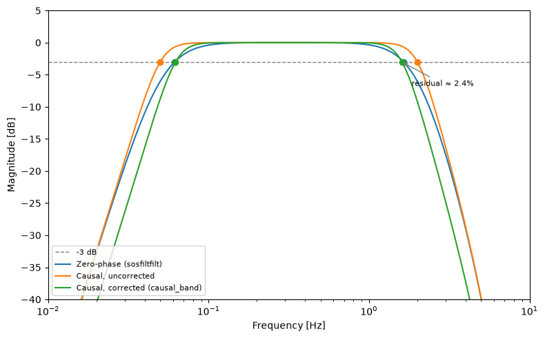
Overlaying the three filter variants
bandpass can produce for a given
freqmin/freqmax/corners: zero-phase, uncorrected causal, and
causal_band-corrected causal. Both causal designs below use
2 * corners poles, matching the rolloff steepness of the
zero-phase filter (sosfiltfilt applies it forward and backward,
doubling the effective order). Parameters use a realistic broadband
passband and sample rate, chosen without tuning to minimise the
visible gap:
>>> import numpy as np
>>> from scipy.signal import iirfilter, sosfreqz
>>> from pysmo.tools.signal import causal_band
>>> freqmin, freqmax, corners = 0.05, 2.0, 2
>>> fs = 20.0
>>> nyquist = fs / 2
>>> freqmin_causal, freqmax_causal = causal_band(freqmin, freqmax, corners)
>>> round(freqmin_causal, 4), round(freqmax_causal, 4)
(0.0623, 1.6045)
>>> sos_zerophase = iirfilter(
...     corners, [freqmin / nyquist, freqmax / nyquist],
...     btype="band", ftype="butter", output="sos",
... )
>>> sos_causal_uncorrected = iirfilter(
...     2 * corners, [freqmin / nyquist, freqmax / nyquist],
...     btype="band", ftype="butter", output="sos",
... )
>>> sos_causal_corrected = iirfilter(
...     2 * corners, [freqmin_causal / nyquist, freqmax_causal / nyquist],
...     btype="band", ftype="butter", output="sos",
... )
>>>
The zero-phase magnitude is the single-pass response squared
(sosfiltfilt applies the filter twice); the causal variants are
the direct single-pass response:
>>> target_db = -20 * np.log10(2**0.5)  # -3.01 dB
>>> def crossing(sos, zerophase, edge_freq, margin=0.6):
...     w, h = sosfreqz(sos, worN=8000, fs=fs)
...     mag = np.abs(h) ** 2 if zerophase else np.abs(h)
...     db = 20 * np.log10(mag + 1e-300)
...     mask = (w > edge_freq * (1 - margin)) & (w < edge_freq * (1 + margin))
...     seg_w, seg_d = w[mask], db[mask] - target_db
...     j = np.where(np.diff(np.sign(seg_d)) != 0)[0]
...     best = j[np.argmin(np.abs(seg_w[j] - edge_freq))]
...     frac = -seg_d[best] / (seg_d[best + 1] - seg_d[best])
...     return seg_w[best] + frac * (seg_w[best + 1] - seg_w[best])
>>> zerophase_edge = crossing(sos_zerophase, True, freqmax)
>>> causal_corrected_edge = crossing(sos_causal_corrected, False, freqmax)
>>> residual_pct = abs(causal_corrected_edge - zerophase_edge) / zerophase_edge * 100
>>> round(float(residual_pct), 1)
2.4
>>>
The corrected marker lands close to the zero-phase one, unlike the
uncorrected marker, which stays at the nominal freqmax=2.0 corner.
A residual of a few percent remains between the corrected and
zero-phase markers (edge interaction, plus some Nyquist-proximity
effect at this sample rate).
Source code in src/pysmo/tools/signal/_filter/_butter.py
132 133 134 135 136 137 138 139 140 141 142 143 144 145 146 147 148 149 150 151 152 153 154 155 156 157 158 159 160 161 162 163 164 165 166 167 168 169 170 171 172 173 174 175 176 177 178 179 180 181 182 183 184 185 186 187 188 189 190 191 192 193 194 195 196 197 198 199 200 201 202 203 204 205 206 207 208 209 210 211 212 213 214 215 216 217 218 219 220 221 222 223 224 225 226 227 228 229 230 231 232 233 234 235 236 237 238 239 240 241 242 243 244 245 246 247 248 249 250 251 252 253 254 255 256 257 258 259 260 261 262 263 264 265 266 267 268 269 270 271 272 273 274 275 276 277 278 279 280 281 282 283 284 285 286 287 288 289 290 291 292 293 294 295 296 297 298 299 300 301 302 303 304 305 306 307 308 309 310 311 312 313 | |
delay(
    seismogram1: Seismogram,
    seismogram2: Seismogram,
    total_delay: bool = False,
    max_shift: NonNegativeTimedelta | None = None,
    abs_max: bool = False,
) -> tuple[Timedelta, float]
Cross correlates two seismograms to determine signal delay.
This function is a wrapper around the correlate
function. The default behaviour is to call the correlate function with
mode="full" using the full length data of the input seismograms.
This is the most robust option, but also the slowest.
If an approximate delay is known (e.g. because a particular phase is being
targeted using a computed arrival time), the search space can be limited
by setting the max_shift parameter to a value. The length of the
seismogram data used for the cross-correlation is then set such that the
calculated delay lies within +/- max_shift.
max_shift ignores begin times
max_shift intentionally does not take the begin times of the
seismograms into consideration. Thus, calling delay() with
total_delay=True may return a delay that is larger than
max_shift.
Implications of setting the max_shift parameter are as follows:
- This mode requires the seismograms to be of equal length.
- If the true delay (i.e. the amount of time the seismograms should be
shifted by) lies within the
max_shiftrange, and also produces the highest correlation, the delay time returned is identical for both methods. - If the true delay lies outside the
max_shiftrange and produces the highest correlation, the delay time returned will be incorrect whenmax_shiftis set. - In the event that the true delay lies within the
max_shiftrange but the maximum signal correlation occurs outside, it will be correctly retrieved when themax_shiftparameter is set, while not setting it yields an incorrect result.
Parameters:
| Name | Type | Description | Default |
|---|---|---|---|
seismogram1
|
Seismogram
|
First seismogram to use for cross correlation. |
required |
seismogram2
|
Seismogram
|
Second seismogram to use for cross correlation. |
required |
total_delay
|
bool
|
Include the difference in |
False
|
max_shift
|
NonNegativeTimedelta | None
|
Maximum (absolute) length of the delay. |
None
|
abs_max
|
bool
|
Return the delay corresponding to absolute maximum. |
False
|
Returns:
| Name | Type | Description |
|---|---|---|
delay |
Timedelta
|
Time delay of the second seismogram with respect to the first. |
cc |
float
|
Normalised cross-correlation value of the overlapping
seismograms after shifting (uses
|
Raises:
| Type | Description |
|---|---|
ValueError
|
If either seismogram has no data, or if |
Examples:
To illustrate the delay() function: this reads a seismogram from a
SAC file, then generates a second seismogram from it with a shift in
the data and in the begin time. That makes the true delay known, so
it can be compared against the computed delay:
>>> from pysmo import MiniSeismogram
>>> from pysmo.classes import SAC
>>> from pysmo.functions import detrend, clone_to_mini
>>> from pysmo.tools.signal import delay
>>> from datetime import timedelta
>>> import numpy as np
>>>
>>> # Create a Seismogram from a SAC file and detrend it:
>>> seis1 = SAC.from_file("example.sac").seismogram
>>> detrend(seis1)
>>>
>>> # Create a second seismogram from the first with
>>> # a different begin_time and a shift in the data:
>>> seis2 = clone_to_mini(MiniSeismogram, seis1)
>>> nroll = 1234
>>> seis2.data = np.roll(seis2.data, nroll)
>>> begin_time_delay = timedelta(seconds=100)
>>> seis2.begin_time += begin_time_delay
>>>
>>> # The signal delay is the number of samples shifted * delta:
>>> (signal_delay := nroll * seis1.delta).total_seconds()
61.7
>>>
>>> # Call the delay function with the two seismograms and verify
>>> # that the caclulated_delay is equal to the known signal delay:
>>> calculated_delay, _ = delay(seis1, seis2)
>>> calculated_delay == signal_delay
True
>>>
Since the true delay is known, this can mimic a scenario where an
approximate delay is known before the cross-correlation, which can be
used to limit the search space and speed up the calculation. Here,
max_shift is set to the known signal delay plus 1 second:
>>> max_shift = signal_delay + timedelta(seconds=1)
>>> calculated_delay, _ = delay(seis1, seis2, max_shift=max_shift)
>>> # As before, the calculated delay should be equal to the signal delay:
>>> calculated_delay == signal_delay
True
>>>
Setting total_delay=True also takes into account the difference
in begin_time between the two seismograms:
>>> calculated_delay, _ = delay(seis1, seis2, total_delay=True, max_shift=signal_delay+timedelta(seconds=1))
>>> # With `total_delay=True`, the calculated delay should be equal to
>>> # the signal delay plus the begin time difference:
>>> calculated_delay == signal_delay + (seis2.begin_time - seis1.begin_time)
True
>>>
To demonstrate the abs_max parameter, the second seismogram's data
is sign-flipped:
>>> seis2.data *= -1
>>> calculated_delay, cc = delay(seis1, seis2)
>>> # Without `abs_max=True`, the calculated delay is no longer equal
>>> # to the true signal delay (as expected):
>>> calculated_delay == signal_delay
False
>>> # The normalised cross-correlation value is also not very high
>>> cc
np.float64(0.5094230)
>>>
>>> calculated_delay, cc = delay(seis1, seis2, abs_max=True)
>>> # with `abs_max=True`, the signal delay is again retrieved:
>>> calculated_delay == signal_delay
True
>>> # And, as the signals are completely opposite, the normalised
>>> # cross-correlation value is -1:
>>> np.testing.assert_approx_equal(cc, -1)
>>>
Source code in src/pysmo/tools/signal/_delay.py
56 57 58 59 60 61 62 63 64 65 66 67 68 69 70 71 72 73 74 75 76 77 78 79 80 81 82 83 84 85 86 87 88 89 90 91 92 93 94 95 96 97 98 99 100 101 102 103 104 105 106 107 108 109 110 111 112 113 114 115 116 117 118 119 120 121 122 123 124 125 126 127 128 129 130 131 132 133 134 135 136 137 138 139 140 141 142 143 144 145 146 147 148 149 150 151 152 153 154 155 156 157 158 159 160 161 162 163 164 165 166 167 168 169 170 171 172 173 174 175 176 177 178 179 180 181 182 183 184 185 186 187 188 189 190 191 192 193 194 195 196 197 198 199 200 201 202 203 204 205 206 207 208 209 210 211 212 213 214 215 216 217 218 219 220 221 222 223 224 225 226 227 228 229 230 231 232 233 234 235 236 237 238 239 240 241 242 243 244 245 246 247 248 249 250 251 252 253 254 255 256 | |
differentiate(
    seismogram: T, *, replace: bool = False
) -> T | None
Differentiate a seismogram in the frequency domain.
Multiplies the FFT of seismogram.data by \(i\omega\) at each
rfftfreq bin, then inverse transforms back to the
time domain. The DC bin is correctly zeroed (\(i\omega = 0\)), since a
constant offset differentiates to zero. For an even-length signal the
Nyquist bin is dropped: irfft requires it to be real, and \(i\omega\)
makes it imaginary.
Parameters:
| Name | Type | Description | Default |
|---|---|---|---|
seismogram
|
T
|
Seismogram object. |
required |
replace
|
bool
|
Return a new seismogram and leave the input untouched,
instead of modifying it in place. Not supported by every
concrete type (see |
False
|
Returns:
| Type | Description |
|---|---|
T | None
|
Differentiated |
T | None
|
|
Raises:
| Type | Description |
|---|---|
ValueError
|
If |
ValueError
|
If |
Examples:
A synthetic sine wave with a known closed-form derivative (\(\omega \cos(\omega t)\)) is used to verify the result:
>>> import numpy as np
>>> import pandas as pd
>>> from pysmo import MiniSeismogram
>>> from pysmo.tools.signal import differentiate
>>> dt = 0.1
>>> npts = 250  # an exact number of cycles of the 1 Hz signal below
>>> t = np.arange(npts) * dt
>>> omega = 2 * np.pi * 1.0
>>> seismogram = MiniSeismogram(
...     begin_time=pd.Timestamp("2010-02-27T06:30:00Z"),
...     delta=pd.Timedelta(seconds=dt),
...     data=np.sin(omega * t),
... )
>>> velocity = differentiate(seismogram, replace=True)
>>> expected = omega * np.cos(omega * t)
>>> np.allclose(velocity.data, expected, atol=1e-6)
True
>>>
Source code in src/pysmo/tools/signal/_calculus.py
Calculate the envelope of a Gaussian-filtered seismogram.
Parameters:
| Name | Type | Description | Default |
|---|---|---|---|
seismogram
|
T
|
Seismogram object. |
required |
fc
|
float
|
Centre frequency of the Gaussian filter (in Hz). |
required |
alpha
|
float
|
Dimensionless shape parameter controlling the filter width. Larger values produce a narrower (more selective) filter. |
required |
replace
|
bool
|
Return a new seismogram and leave the input untouched,
instead of modifying it in place. Not supported by every
concrete type (see |
False
|
Returns:
| Type | Description |
|---|---|
T | None
|
Seismogram containing the envelope. |
Raises:
| Type | Description |
|---|---|
ValueError
|
If |
Examples:
>>> from pysmo.classes import MSeed
>>> from pysmo.tools.signal import envelope
>>> seis = MSeed.from_file("example.mseed")
>>> fc = 0.02 # Centre Gaussian filter at 0.02 Hz (50s period)
>>> alpha = 50 # Set alpha (which determines filterwidth) to 50
>>> envelope_seis = envelope(seis, fc, alpha, replace=True)
>>>
Source code in src/pysmo/tools/signal/_filter/_gauss.py
filter(
    seismogram: T,
    filter_name: FilterName,
    *,
    replace: bool = False,
    **filter_options: bool | int | float
) -> T | None
Apply a specified filter to the input seismogram.
This function is a convenience wrapper that calls other filters in this module.
Parameters:
| Name | Type | Description | Default |
|---|---|---|---|
seismogram
|
T
|
The input seismogram to be filtered. |
required |
filter_name
|
FilterName
|
The type of filter to apply. |
required |
replace
|
bool
|
If |
False
|
**filter_options
|
bool | int | float
|
Filter parameters passed to the specified filter function. |
{}
|
Returns:
| Type | Description |
|---|---|
T | None
|
A new Seismogram containing the filtered data when called with |
T | None
|
|
Raises:
| Type | Description |
|---|---|
ValueError
|
If |
Examples:
>>> from pysmo.classes import MSeed
>>> from pysmo.tools.signal import filter
>>> seis = MSeed.from_file("example.mseed")
>>>
>>> # create a new filtered seismogram with a lowpass filter
>>> filtered_seis = filter(seis, "lowpass", freqmax=0.5, replace=True)
>>>
>>> # or update in place with a bandpass filter
>>> filter(seis, "bandpass", freqmin=0.1, freqmax=0.5)
>>>
Source code in src/pysmo/tools/signal/_filter/_filter.py
Return a Gaussian-filtered seismogram.
Parameters:
| Name | Type | Description | Default |
|---|---|---|---|
seismogram
|
T
|
Seismogram object. |
required |
fc
|
float
|
Centre frequency of the Gaussian filter (in Hz). |
required |
alpha
|
float
|
Dimensionless shape parameter controlling the filter width. Larger values produce a narrower (more selective) filter. |
required |
replace
|
bool
|
Return a new seismogram and leave the input untouched,
instead of modifying it in place. Not supported by every
concrete type (see |
False
|
Returns:
| Type | Description |
|---|---|
T | None
|
Gaussian-filtered seismogram. |
Raises:
| Type | Description |
|---|---|
ValueError
|
If |
Examples:
>>> from pysmo.classes import MSeed
>>> from pysmo.tools.signal import gauss
>>> seis = MSeed.from_file("example.mseed")
>>> fc = 0.02 # Centre Gaussian filter at 0.02 Hz (50s period)
>>> alpha = 50 # Set alpha (which determines filterwidth) to 50
>>> gauss_seis = gauss(seis, fc, alpha, replace=True)
>>>
Source code in src/pysmo/tools/signal/_filter/_gauss.py
highpass(
    seismogram: T,
    freqmin: float = 0.1,
    corners: PositiveInt = 2,
    zerophase: bool = False,
    *,
    replace: bool = False
) -> T | None
Apply a highpass filter to the input seismogram.
Parameters:
| Name | Type | Description | Default |
|---|---|---|---|
seismogram
|
T
|
The input seismogram to be filtered. |
required |
freqmin
|
float
|
The minimum frequency of the highpass filter (in Hz). |
0.1
|
corners
|
PositiveInt
|
The number of corners (poles) for the Butterworth filter. |
2
|
zerophase
|
bool
|
If |
False
|
replace
|
bool
|
If |
False
|
Returns:
| Type | Description |
|---|---|
T | None
|
A new Seismogram containing the filtered data when called with |
T | None
|
|
Raises:
| Type | Description |
|---|---|
ValueError
|
If |
Source code in src/pysmo/tools/signal/_filter/_butter.py
integrate(
    seismogram: T, *, replace: bool = False
) -> T | None
Integrate a seismogram in the frequency domain.
Divides the FFT of seismogram.data by \(i\omega\) at each
rfftfreq bin (\(\omega > 0\)), then inverse
transforms back to the time domain. The DC bin is set to 0.0 rather
than divided by. For an even-length signal the Nyquist bin is dropped:
irfft requires it to be real, and dividing by \(i\omega\) makes it
imaginary. Working in the frequency domain avoids the unbounded
low-frequency drift a cumulative time-domain integrator introduces.
Parameters:
| Name | Type | Description | Default |
|---|---|---|---|
seismogram
|
T
|
Seismogram object. |
required |
replace
|
bool
|
Return a new seismogram and leave the input untouched,
instead of modifying it in place. Not supported by every
concrete type (see |
False
|
Returns:
| Type | Description |
|---|---|
T | None
|
Integrated |
T | None
|
|
Raises:
| Type | Description |
|---|---|
ValueError
|
If |
ValueError
|
If |
Examples:
A synthetic cosine wave with a known closed-form integral (\(\sin(\omega t)\)) is used to verify the result:
>>> import numpy as np
>>> import pandas as pd
>>> from pysmo import MiniSeismogram
>>> from pysmo.tools.signal import integrate
>>> dt = 0.1
>>> npts = 250  # an exact number of cycles of the 1 Hz signal below
>>> t = np.arange(npts) * dt
>>> omega = 2 * np.pi * 1.0
>>> seismogram = MiniSeismogram(
...     begin_time=pd.Timestamp("2010-02-27T06:30:00Z"),
...     delta=pd.Timedelta(seconds=dt),
...     data=omega * np.cos(omega * t),
... )
>>> displacement = integrate(seismogram, replace=True)
>>> expected = np.sin(omega * t)
>>> np.allclose(displacement.data, expected, atol=1e-6)
True
>>>
Source code in src/pysmo/tools/signal/_calculus.py
lowpass(
    seismogram: T,
    freqmax: float = 0.5,
    corners: PositiveInt = 2,
    zerophase: bool = False,
    *,
    replace: bool = False
) -> T | None
Apply a lowpass filter to the input seismogram.
Parameters:
| Name | Type | Description | Default |
|---|---|---|---|
seismogram
|
T
|
The input seismogram to be filtered. |
required |
freqmax
|
float
|
The maximum frequency of the lowpass filter (in Hz). |
0.5
|
corners
|
PositiveInt
|
The number of corners (poles) for the Butterworth filter. |
2
|
zerophase
|
bool
|
If |
False
|
replace
|
bool
|
If |
False
|
Returns:
| Type | Description |
|---|---|
T | None
|
A new Seismogram containing the filtered data when called with |
T | None
|
|
Raises:
| Type | Description |
|---|---|
ValueError
|
If |
Source code in src/pysmo/tools/signal/_filter/_butter.py
mccc(
    seismograms: Sequence[Seismogram],
    min_cc: float = 0.5,
    damping: float = 0.1,
    abs_max: bool = False,
) -> tuple[
    list[Timedelta],
    list[Timedelta | None],
    Timedelta,
    list[float],
    list[float],
]
Multi-Channel Cross-Correlation (MCCC) for relative arrival times.
Computes all pairwise cross-correlation delays using
multi_multi_delay, then solves
for self-consistent relative time shifts using a weighted least-squares
inversion with a zero-mean constraint and Tikhonov regularisation. Pairs
whose correlation coefficient falls below min_cc are excluded from the
inversion.
The returned times list sums to zero by construction, so the values
represent relative shifts around the group mean.
Parameters:
| Name | Type | Description | Default |
|---|---|---|---|
seismograms
|
Sequence[Seismogram]
|
Sequence of Seismogram objects. All must share the same sampling interval. |
required |
min_cc
|
float
|
Minimum correlation coefficient required to include a pair in the inversion. |
0.5
|
damping
|
float
|
Tikhonov regularisation strength. Set to 0 to disable. |
0.1
|
abs_max
|
bool
|
If |
False
|
Returns:
| Name | Type | Description |
|---|---|---|
times |
list[Timedelta]
|
List of relative arrival times. |
errors |
list[Timedelta | None]
|
List of standard errors. If the weighted normal-equations
matrix is singular (e.g. too few correlated pairs relative to
|
rmse |
Timedelta
|
Root-mean-square error of the fit. |
cc_means |
list[float]
|
Mean correlation coefficient for each seismogram. |
cc_stds |
list[float]
|
Standard deviation of correlation coefficients for each seismogram. |
Raises:
| Type | Description |
|---|---|
ValueError
|
If any seismogram has a different sampling rate than the
others (raised by |
Notes
The returned statistics provide key diagnostic information:
- Cycle Skip: High errors combined with high cc_means and low
cc_stds suggests a cycle skip (the waveform matches perfectly but
on the wrong peak).
- Noisy Seismogram: Low cc_means combined with high errors and
cc_stds indicates poor data quality or significant site-response
distortion.
- Array Coherence: The rmse measures the overall fit. High rmse
even with high cc_means suggests the array is too large or sparse
for a single coherent arrival time (e.g., crossing a major tectonic
boundary).
Examples:
Create seismograms with known shifts and recover them with mccc:
>>> from pysmo import MiniSeismogram
>>> from pysmo.tools.signal import mccc
>>> import numpy as np
>>>
>>> # Build three seismograms with known shifts (in samples):
>>> data = np.sin(np.linspace(0, 8 * np.pi, 1000))
>>> shifts = [0, 5, -10]
>>> seismograms = [MiniSeismogram(data=np.roll(data, s)) for s in shifts]
>>>
>>> # Run MCCC inversion:
>>> times, errors, rmse, cc, cc_std = mccc(seismograms)
>>>
>>> # The relative times sum to approximately zero:
>>> abs(sum(t.total_seconds() for t in times)) < 1e-5
True
>>>
>>> # Pairwise differences recover the known shifts
>>> # (times[i] - times[j] ≈ (shifts[i] - shifts[j]) * delta):
>>> round((times[1] - times[0]).total_seconds())
5
>>> round((times[2] - times[0]).total_seconds())
-10
>>>
Use abs_max=True to recover shifts for polarity-flipped signals:
>>> # Create a set of seismograms where one has inverted polarity:
>>> seismograms[1].data *= -1
>>>
>>> # Run MCCC with abs_max=True:
>>> times, errors, rmse, cc, cc_std = mccc(seismograms, abs_max=True)
>>>
>>> # Shifts are still correctly recovered:
>>> round((times[1] - times[0]).total_seconds())
5
>>> # The correlation coefficient for the flipped signal is negative:
>>> cc[1] < -0.9
True
>>>
References
VanDecar, J. C., and R. S. Crosson. “Determination of Teleseismic Relative Phase Arrival Times Using Multi-Channel Cross-Correlation and Least Squares.” Bulletin of the Seismological Society of America, vol. 80, no. 1, Feb. 1990, pp. 150–69, https://doi.org/10.1785/BSSA0800010150.
Source code in src/pysmo/tools/signal/_delay.py
595 596 597 598 599 600 601 602 603 604 605 606 607 608 609 610 611 612 613 614 615 616 617 618 619 620 621 622 623 624 625 626 627 628 629 630 631 632 633 634 635 636 637 638 639 640 641 642 643 644 645 646 647 648 649 650 651 652 653 654 655 656 657 658 659 660 661 662 663 664 665 666 667 668 669 670 671 672 673 674 675 676 677 678 679 680 681 682 683 684 685 686 687 688 689 690 691 692 693 694 695 696 697 698 699 700 701 702 703 704 705 706 707 708 709 710 711 712 713 714 715 716 717 718 719 720 721 722 723 724 725 726 727 728 729 730 731 732 733 734 735 736 737 738 739 740 741 742 743 744 745 746 747 748 749 750 751 752 753 754 755 756 757 758 759 760 761 762 763 764 765 766 767 768 769 770 771 772 773 774 775 776 777 778 779 780 781 782 783 784 785 786 787 788 789 790 791 792 793 794 795 796 797 798 799 800 801 802 803 804 805 806 807 808 809 810 811 812 | |
multi_delay(
    template: Seismogram,
    seismograms: Sequence[Seismogram],
    abs_max: bool = False,
    max_shift: NonNegativeTimedelta | None = None,
) -> tuple[list[Timedelta], list[float]]
Compute delays and correlation coefficients for many seismograms vs a template.
This function uses FFT-based cross-correlation to efficiently compute delays
for multiple seismograms at once against a single template. This is faster
than calling delay in a loop, as the template
FFT is computed only once.
Parameters:
| Name | Type | Description | Default |
|---|---|---|---|
template
|
Seismogram
|
Template seismogram object. |
required |
seismograms
|
Sequence[Seismogram]
|
Sequence of Seismogram objects. |
required |
abs_max
|
bool
|
If |
False
|
max_shift
|
NonNegativeTimedelta | None
|
Maximum (absolute) shift to consider. If set, the search for
the maximum correlation is restricted to lags within |
None
|
Returns:
| Name | Type | Description |
|---|---|---|
delays |
list[Timedelta]
|
Delays of each input seismogram relative to template. |
ccs |
list[float]
|
Correlation coefficients at maximum correlation for each seismogram. |
Raises:
| Type | Description |
|---|---|
ValueError
|
If any seismogram has a different sampling rate than the template. |
ValueError
|
If |
ValueError
|
If the template or any seismogram has no data. |
Differs from delay()
Unlike delay, max_shift here does not
require the seismograms to be of equal length, and does not speed up
the calculation (the full cross-correlation is always computed; only
the search for its maximum is restricted). If the true delay lies
outside the max_shift range, the delay returned will be constrained
to (and typically found at the edge of) that range, and its
correlation coefficient will usually be low.
Constant-data seismograms cannot be normalised
Seismograms with zero standard deviation (i.e. constant data) cannot be
meaningfully normalised. A UserWarning is issued for each such trace and
its normalised values are treated as zero, which results in a correlation
coefficient of 0 for that trace. In an MCCC workflow this effectively
excludes the trace from the inversion via the min_cc threshold.
Examples:
Create a template seismogram and several shifted copies, then use
multi_delay to recover the known shifts:
>>> from pysmo import MiniSeismogram
>>> from pysmo.tools.signal import multi_delay
>>> import numpy as np
>>>
>>> # Create a template seismogram with sinusoidal data:
>>> data = np.sin(np.linspace(0, 8 * np.pi, 1000))
>>> template = MiniSeismogram(data=data)
>>>
>>> # Create shifted copies (shifts in samples):
>>> shifts = [0, 10, -5]
>>> seismograms = [MiniSeismogram(data=np.roll(data, s)) for s in shifts]
>>>
>>> # Calculate delays for all seismograms at once:
>>> delays, ccs = multi_delay(template, seismograms)
>>> [d.total_seconds() for d in delays]
[0.0, 10.0, -5.0]
>>>
Use abs_max=True for polarity-insensitive matching:
>>> flipped = MiniSeismogram(data=-np.roll(data, 10))
>>> delays, ccs = multi_delay(template, [flipped], abs_max=True)
>>> delays[0].total_seconds()
10.0
>>> ccs[0] < 0
True
>>>
Use max_shift to restrict the search space, e.g. to avoid a spurious
match at a larger, unwanted lag:
>>> import pandas as pd
>>> shifted = MiniSeismogram(data=np.roll(data, 10))
>>> delays, ccs = multi_delay(
...     template, [shifted], max_shift=pd.Timedelta(seconds=20)
... )
>>> delays[0].total_seconds()
10.0
>>>
Source code in src/pysmo/tools/signal/_delay.py
259 260 261 262 263 264 265 266 267 268 269 270 271 272 273 274 275 276 277 278 279 280 281 282 283 284 285 286 287 288 289 290 291 292 293 294 295 296 297 298 299 300 301 302 303 304 305 306 307 308 309 310 311 312 313 314 315 316 317 318 319 320 321 322 323 324 325 326 327 328 329 330 331 332 333 334 335 336 337 338 339 340 341 342 343 344 345 346 347 348 349 350 351 352 353 354 355 356 357 358 359 360 361 362 363 364 365 366 367 368 369 370 371 372 373 374 375 376 377 378 379 380 381 382 383 384 385 386 387 388 389 390 391 392 393 394 395 396 397 398 399 400 401 402 403 404 405 406 407 408 409 410 411 412 413 414 415 416 417 418 419 420 421 422 423 424 425 426 427 428 429 430 431 432 433 434 435 436 437 438 439 440 441 442 443 444 445 | |
multi_multi_delay(
    seismograms: Sequence[Seismogram], abs_max: bool
) -> tuple[NDArray[timedelta64], NDArray[floating]]
Compute pairwise delays and correlation coefficients for a set of seismograms.
This function cross-correlates every seismogram with every other seismogram
in the sequence using FFT-based cross-correlation. All FFTs are computed once
and combined via broadcasting, making this significantly faster than calling
delay for each pair individually.
The result at delays[i, j] is the delay of seismogram j relative to
seismogram i (treating i as the reference). The diagonal is zero and
the matrix is antisymmetric (delays[i, j] == -delays[j, i]), except where
the two directions' correlation peaks disagree by a sample, as can happen
for near-periodic or multi-peak waveforms. Each cc_matrix entry is the
correlation at its own cell's chosen lag.
Returns numpy.timedelta64, not Timedelta
Unlike most pysmo functions, this returns numpy.timedelta64 values
rather than Timedelta. This avoids the overhead
of an object array and allows efficient vectorised arithmetic in
downstream functions such as mccc.
Convert individual elements with pandas.Timedelta(delays[i, j]) if
needed.
Parameters:
| Name | Type | Description | Default |
|---|---|---|---|
seismograms
|
Sequence[Seismogram]
|
Sequence of Seismogram objects. |
required |
abs_max
|
bool
|
If |
required |
Returns:
| Name | Type | Description |
|---|---|---|
delays |
NDArray[timedelta64]
|
2D array of shape |
cc_matrix |
NDArray[floating]
|
2D array of shape |
Raises:
| Type | Description |
|---|---|
ValueError
|
If any seismogram has a different sampling rate than the others. |
ValueError
|
If any seismogram has no data. |
Constant-data seismograms cannot be normalised
Seismograms with zero standard deviation (i.e. constant data) cannot be
meaningfully normalised. A UserWarning is issued for each such trace and
its normalised values are treated as zero, resulting in correlation
coefficients of 0 for all pairs involving that trace.
Examples:
Create seismograms with known shifts and compute all pairwise delays:
>>> from pysmo import MiniSeismogram
>>> from pysmo.tools.signal import multi_multi_delay
>>> import pandas as pd
>>> import numpy as np
>>>
>>> data = np.sin(np.linspace(0, 8 * np.pi, 1000))
>>> seismograms = [
...     MiniSeismogram(data=data.copy()),
...     MiniSeismogram(data=np.roll(data, 5)),
...     MiniSeismogram(data=np.roll(data, -10)),
... ]
>>>
>>> delays, cc_matrix = multi_multi_delay(seismograms, abs_max=False)
>>> delays.shape
(3, 3)
>>> # delay of seismogram 1 relative to seismogram 0:
>>> pd.Timedelta(delays[0, 1]).total_seconds()
5.0
>>> # delay of seismogram 2 relative to seismogram 0:
>>> pd.Timedelta(delays[0, 2]).total_seconds()
-10.0
>>> # antisymmetric: delays[i, j] == -delays[j, i]
>>> pd.Timedelta(delays[1, 0]).total_seconds()
-5.0
>>>
Source code in src/pysmo/tools/signal/_delay.py
448 449 450 451 452 453 454 455 456 457 458 459 460 461 462 463 464 465 466 467 468 469 470 471 472 473 474 475 476 477 478 479 480 481 482 483 484 485 486 487 488 489 490 491 492 493 494 495 496 497 498 499 500 501 502 503 504 505 506 507 508 509 510 511 512 513 514 515 516 517 518 519 520 521 522 523 524 525 526 527 528 529 530 531 532 533 534 535 536 537 538 539 540 541 542 543 544 545 546 547 548 549 550 551 552 553 554 555 556 557 558 559 560 561 562 563 564 565 566 567 568 569 570 571 572 573 574 575 576 577 578 579 580 581 582 583 584 585 586 587 588 589 590 591 592 | |
psd(
    seismogram: Seismogram,
    nperseg: int,
    nfft: int,
    scaling: Literal["density", "spectrum"] = "density",
    include_dc: bool = False,
) -> tuple[NDArray[floating], NDArray[floating]]
Calculate the Power Spectral Density (PSD) of a Seismogram using Welch's method.
This is a convenience wrapper around welch.
Parameters:
| Name | Type | Description | Default |
|---|---|---|---|
seismogram
|
Seismogram
|
The Seismogram object. |
required |
nperseg
|
int
|
Length of each segment for Welch's method. |
required |
nfft
|
int
|
Length of the FFT used. |
required |
scaling
|
Literal['density', 'spectrum']
|
The scaling method for the PSD. |
'density'
|
include_dc
|
bool
|
If |
False
|
Returns:
| Type | Description |
|---|---|
tuple[NDArray[floating], NDArray[floating]]
|
A tuple containing the frequencies and the Power Spectral Density. |
Source code in src/pysmo/tools/signal/_spectral.py
remove_response(
    seismogram: T,
    response: Response,
    pre_filt: (
        tuple[float, float, float, float] | None
    ) = None,
    *,
    replace: bool = False
) -> T | None
Remove an instrument response from a seismogram.
Two modes are available, chosen by whether pre_filt is given:
pre_filt=None (default): sensitivity-only division. Divides
seismogram.data by response.reference_sensitivity alone, in the time
domain. No FFT, no frequency-dependent correction: this is only correct
where the true instrument response is flat with \(\approx 0\) phase, i.e. within
the sensor's own passband, and is appropriate when the signal of interest
is confined to that flat band (the common case for a well-chosen broadband
instrument). It will not correct roll-off near the sensor's corner
frequencies or any digital decimation stages; for that, use pre_filt.
Note this divides by reference_sensitivity, not overall_sensitivity;
the latter has the analog stage's \(A_0\) normalisation factor folded in (see
Response.overall_sensitivity).
For a SacPZ-derived response, this path's output
is typically not in the units input_units declares: by SAC convention
(followed by e.g. EarthScope's fdsnws-station service and rdseed -p), the
SENSITIVITY header (reference_sensitivity) stays in the sensor's
native units (e.g. M/S**2 for an accelerometer), while
poles/zeros/overall_sensitivity (and therefore input_units, and
the full-deconvolution path below) are normalised to displacement. This
is a convention of the producer, not something SacPZ/parse_sacpz
enforce or verify; a hand-written SAC PZ file that doesn't follow it will
not exhibit this split. A StationXML-derived
response has no such split: both paths agree with input_units.
pre_filt given: spectral deconvolution. Deconvolves seismogram.data
by the instrument response's full complex transfer function \(H(f)\),
applying a four-corner cosine taper \(\text{taper}(f)\):
The effective filter response \(\frac{\text{taper}(f)}{H(f)}\) is forced to zero outside \((f_1, f_4)\) (skipping division by \(H(f)\) where \(\text{taper}(f) = 0\)), and cosine-tapered at the edges (\(f_1 < f_2 \le f_3 < f_4\), in Hz), so frequencies excluded from the passband are never amplified. There is no additional stabilisation: if \(H(f)\) is zero or very small at a frequency inside \((f_1, f_4)\), division amplifies noise without limit, and an exact zero produces non-finite values (\(\infty\) or \(\text{NaN}\)) that poison the entire output once inverse-transformed. Consequently, \(f_1\) must remain strictly above 0 Hz, since velocity- and acceleration-output sensors have a zero at DC by construction (2 or 3 zeros at the origin, respectively; that is what makes it a velocity/acceleration sensor, not a displacement one).
The right bound for \(f_4\) also depends on whether response actually carries
digital FIR/IIR decimation stages, not just whether it satisfies
StagedResponse, since e.g.
StationXML.response always
satisfies that protocol but its stages is empty for a document with no
digital stage on record:
- No digital stages (
stagesempty, e.g. a SAC PZ-derived response, or a StationXML document without one): only the analog poles/zeros/sensitivity go into \(H(f)\). Pushing \(f_4\) above roughly 80% of the seismogram's own Nyquist frequency triggers theUserWarningdescribed below; the analog-only approximation ignores the roll-off and phase a real digitiser's decimation filter would otherwise contribute near its own Nyquist. - Digital stages present (
stagesnon-empty): they are folded into \(H(f)\) too, so \(f_4\) should also stay clear of their own cutoff: bound it by the stages' own Nyquist (half theirinput_sample_rate), not just the seismogram's, since a stage's own zeros cluster in its stopband near/above that frequency. Stages are also assumed to have had their own filter delay already corrected out of the recorded data (ResponseStage.correction, matching FDSN StationXML'sDecimation/Correction, as is standard for archived data); if that assumption doesn't hold for a givenresponse, the deconvolved output will carry a spurious time shift equal to that correction.
No other preprocessing is performed in the deconvolution path:
seismogram.data is not zero-padded, demeaned, detrended, or tapered in
the time domain before the FFT. Since rfft/irfft implicitly treat
the data as one period of a periodic signal, an uncorrected mean/trend
or an abrupt jump between the segment's start and end will produce
wraparound artefacts in the deconvolved output rather than being cleanly
removed. Detrend and taper the seismogram first (e.g. with
pysmo.functions.detrend and
pysmo.functions.taper), as is standard
practice before any FFT-based deconvolution.
Parameters:
| Name | Type | Description | Default |
|---|---|---|---|
seismogram
|
T
|
The seismogram to deconvolve. |
required |
response
|
Response
|
The instrument response to remove. Output is in whatever
physical units |
required |
pre_filt
|
tuple[float, float, float, float] | None
|
Optional four corner frequencies \((f_1, f_2, f_3, f_4)\) in Hz
defining a cosine taper applied before division: zero below
\(f_1\), cosine ramp up to \(f_2\), flat through \([f_2, f_3]\), cosine
ramp down to \(f_4\), zero above \(f_4\). |
None
|
replace
|
bool
|
Return a new seismogram and leave the input untouched,
instead of modifying it in place. Not supported by every
concrete type (see |
False
|
Returns:
| Type | Description |
|---|---|
T | None
|
Processed |
T | None
|
|
Raises:
| Type | Description |
|---|---|
ValueError
|
If |
Warns:
| Type | Description |
|---|---|
UserWarning
|
If |
Examples:
The examples below build on the same setup: example.mseed's own real
response: a broadband seismometer and digitiser, from a genuine StationXML
document for the actual station and epoch that recorded it.
Sensitivity-only division:
>>> from pathlib import Path
>>> from pysmo.classes import MSeed, StationXML
>>> from pysmo.tools.signal import remove_response
>>> xml = Path("example_response.xml").read_bytes()
>>> original = MSeed.from_file("example.mseed")
>>> response = StationXML.from_bytes(xml, time=original.begin_time).response
>>> seismogram = remove_response(original, response, replace=True)
>>> len(seismogram.data) == len(original.data)
True
>>>
Full spectral deconvolution, detrended and tapered first to avoid the
wraparound artefacts described above. \(f_4\) is bounded by both the
seismogram's own Nyquist and the digital stages' (a stage is only meaningful
up to half its own input_sample_rate); \(f_1\) is read off the analog poles'
own corner, below which deconvolution mostly amplifies sensor noise. Neither
bound is computed automatically; the right choice is study-dependent (e.g.
teleseismic earthquakes vs. ambient noise), so this is left to the caller:
>>> from pysmo.functions import detrend, taper
>>> nyquist = 0.5 / original.delta.total_seconds()
>>> stage_nyquist = min(stage.input_sample_rate / 2 for stage in response.stages)
>>> f4 = 0.8 * min(nyquist, stage_nyquist)
>>> f3 = f4 * 0.9
>>> f1 = min(abs(pole) for pole in response.poles if pole != 0) / 10
>>> f2 = f1 * 10
>>> pre_filt = (f1, f2, f3, f4)
>>> prepped = detrend(original, replace=True)
>>> taper(prepped, 0.05)
>>> deconvolved = remove_response(prepped, response, pre_filt=pre_filt, replace=True)
>>> len(deconvolved.data) == len(original.data)
True
>>>
Check the data, not just the instrument
\(f_1\)–\(f_4\) above are chosen from the instrument and the
sampling rate, but deconvolution divides by the response
across that whole band, so what actually determines whether the
result is trustworthy is the data's own amplitude at each of
those frequencies, not just where the instrument and sample
rate look reasonable on paper. A technically-defensible
pre_filt can still amplify noise into a poor result if the
data itself has little real amplitude somewhere within that
band.
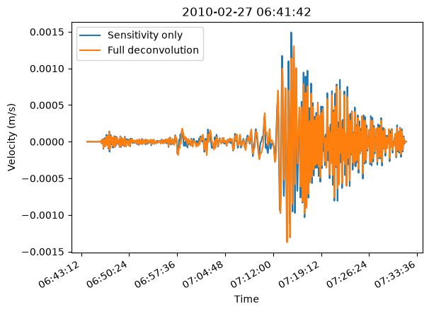
With the earthquake's own dominant period band sitting well within
response's flat passband, the sensitivity-only and full-deconvolution paths
agree closely in both amplitude and shape:
>>> import numpy as np
>>> import pytest
>>> gain_only = remove_response(prepped, response, replace=True)
>>> gain_only_rms = np.sqrt(np.mean(gain_only.data**2))
>>> deconvolved_rms = np.sqrt(np.mean(deconvolved.data**2))
>>> # ~1: amplitude match
>>> float(gain_only_rms / deconvolved_rms) == pytest.approx(1.0, abs=0.15)
True
>>> # ~1: shape match
>>> float(np.corrcoef(gain_only.data, deconvolved.data)[0, 1]) == pytest.approx(1.0, abs=0.15)
True
>>>
Seeing the two paths plotted together makes that agreement concrete rather than abstract:
>>> from pysmo.tools.plotutils import plotseis
>>> fig = plotseis(gain_only, deconvolved)
>>> _ = fig.gca().set_ylabel(f"Velocity ({response.input_units})")
>>> _ = fig.gca().legend(["Sensitivity only", "Full deconvolution"])
>>>
Source code in src/pysmo/tools/signal/_response.py
92 93 94 95 96 97 98 99 100 101 102 103 104 105 106 107 108 109 110 111 112 113 114 115 116 117 118 119 120 121 122 123 124 125 126 127 128 129 130 131 132 133 134 135 136 137 138 139 140 141 142 143 144 145 146 147 148 149 150 151 152 153 154 155 156 157 158 159 160 161 162 163 164 165 166 167 168 169 170 171 172 173 174 175 176 177 178 179 180 181 182 183 184 185 186 187 188 189 190 191 192 193 194 195 196 197 198 199 200 201 202 203 204 205 206 207 208 209 210 211 212 213 214 215 216 217 218 219 220 221 222 223 224 225 226 227 228 229 230 231 232 233 234 235 236 237 238 239 240 241 242 243 244 245 246 247 248 249 250 251 252 253 254 255 256 257 258 259 260 261 262 263 264 265 266 267 268 269 270 271 272 273 274 275 276 277 278 279 280 281 282 283 284 285 286 287 288 289 290 291 292 293 294 295 296 297 298 299 300 301 302 303 304 305 306 307 308 309 310 311 312 313 314 315 316 317 318 319 320 321 322 323 324 325 326 327 328 329 330 331 332 333 334 335 336 337 338 339 340 341 342 343 344 345 346 347 348 349 350 351 352 353 354 355 356 357 358 359 360 361 362 363 364 365 366 367 368 369 370 371 372 373 374 375 376 377 378 379 380 381 382 383 384 385 386 387 388 389 390 391 392 393 394 395 396 397 398 399 400 401 402 403 404 405 406 407 408 409 410 411 412 413 414 415 416 417 418 419 420 421 422 423 424 425 426 427 428 429 430 431 432 433 434 435 436 437 438 439 440 441 442 443 444 445 | |
Corner frequencies so a zero-phase filter's -3dB point matches a causal one's.
The exact inverse of causal_band:
use this when you have causal (single-pass) design frequencies already
chosen (from an existing causal filtering workflow, or from
causal_band itself) and want the zero-phase nominal frequencies whose
actual passband matches them, independent of any particular application.
Converts causal design corner frequencies to the wider nominal frequencies a zero-phase filter needs so that its actual (inward-shifted) -3dB point lands close to the causal filter's actual (nominal) -3dB point.
The inverse is exact and closed-form: the same ratio causal_band
uses, with multiplication and division swapped, not an approximation
or an iterative solve. Both corrected edges move outward from the input band,
the opposite direction from causal_band. The same close-but-not-exact
caveat documented on causal_band applies here too: matching -3dB
points between a digital causal and zero-phase Butterworth bandpass
filter is close, not exact.
Parameters:
| Name | Type | Description | Default |
|---|---|---|---|
freqmin
|
float
|
Causal design minimum frequency (in Hz). |
required |
freqmax
|
float
|
Causal design maximum frequency (in Hz). |
required |
corners
|
PositiveInt
|
The zero-phase filter's number of corners (poles), the
same |
required |
Returns:
| Type | Description |
|---|---|
float
|
The |
float
|
zero-phase filter, with |
tuple[float, float]
|
from the input values. |
Examples:
Round-trip with causal_band recovers the original band exactly:
>>> from pysmo.tools.signal import causal_band, zerophase_band
>>> band = (0.05, 2.0)
>>> corners = 2
>>> causal = causal_band(*band, corners)
>>> recovered = zerophase_band(*causal, corners)
>>> [round(f, 10) for f in recovered]
[0.05, 2.0]